Excel help - if then
Discussion


I have a spreadsheet where the user is answering questions with 5 columns being the Likert scale from strongly agree to strongly disagree, I want to colour the cells in another column further along based on the answers to the questions so the cell goes green if they answer agree, amber if neither and red if disagree for example.
Im not sure I can do that with conditional formatting, will it require a macro?
Im not sure I can do that with conditional formatting, will it require a macro?
Conditional formatting can do it. Select "New Rule" rather than predefined ones, and one of the options is to use a formula. Put in "=A1=1" (or =A1="Agree" if you're using text dropdowns) and then apply the formatting. You can have multiple conditional formats on a single cell so just have 5 to give the different colours (or 4 with the default being the 5th colour)
ETA: Just realised you mean they put something in one of 5 columns rather than a score. As above converting to a number works. If you're using True and False, it stores them as 1 or 0, so you could do a sum product with a list of 1 to 5 so if there's a true in column 3 it returns the number 3.
ETA: Just realised you mean they put something in one of 5 columns rather than a score. As above converting to a number works. If you're using True and False, it stores them as 1 or 0, so you could do a sum product with a list of 1 to 5 so if there's a true in column 3 it returns the number 3.
Edited by RizzoTheRat on Friday 16th July 10:25
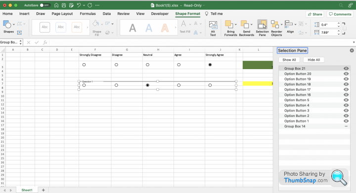
I would put a Group Box (from the Developer Tab, Insert, Form Controls) across all five responses, then five Option Buttons (again from the Developer Tab, Insert, Form Controls), with the option buttons all pointed at the cell in which you want to display the result.
I am going to assume that column A contains the question, then B-F are strongly disagree to strongly agree, then G has the colour code, like this (but line things up nicely):

Select G2, hit Conditional Formatting, New Rule, Use a formula, and then you'll need to do this three times:
First one - formula is "=G2<3", and hit the format button, set the fill to red
Second one - formula is "=G2=3", format button, fill to amber (or maybe yellow)
Third one - formula is "=g2>3", format button, fill to green
That should look like this:

You'll then just need to copy that all down your questions. I'm not sure Excel is the best tool for this, but as with many things, it may be the least bad tool you've got...
I am going to assume that column A contains the question, then B-F are strongly disagree to strongly agree, then G has the colour code, like this (but line things up nicely):
Select G2, hit Conditional Formatting, New Rule, Use a formula, and then you'll need to do this three times:
First one - formula is "=G2<3", and hit the format button, set the fill to red
Second one - formula is "=G2=3", format button, fill to amber (or maybe yellow)
Third one - formula is "=g2>3", format button, fill to green
That should look like this:
You'll then just need to copy that all down your questions. I'm not sure Excel is the best tool for this, but as with many things, it may be the least bad tool you've got...
Sporky said:
I'm not sure Excel is the best tool for this, but as with many things, it may be the least bad tool you've got...
Thats exactly it. If it works for what we need it for after a proof of concept we may be able to shift it to something more suitableThanks for the explanation ill give it a go. Thanks everyone ill come back if I get stuck
craigjm said:
Sporky said:
I'm not sure Excel is the best tool for this, but as with many things, it may be the least bad tool you've got...
Thats exactly it. If it works for what we need it for after a proof of concept we may be able to shift it to something more suitable(35yrs in IT)
This will still be a supported legacy application (spreadsheet) when you retire.. look around you, one day lad, all this will be yours.. what the macros?!

Sporky said:
I would put a Group Box (from the Developer Tab, Insert, Form Controls) across all five responses, then five Option Buttons (again from the Developer Tab, Insert, Form Controls), with the option buttons all pointed at the cell in which you want to display the result.
I am going to assume that column A contains the question, then B-F are strongly disagree to strongly agree, then G has the colour code, like this (but line things up nicely):
Select G2, hit Conditional Formatting, New Rule, Use a formula, and then you'll need to do this three times:
First one - formula is "=G2<3", and hit the format button, set the fill to red
Second one - formula is "=G2=3", format button, fill to amber (or maybe yellow)
Third one - formula is "=g2>3", format button, fill to green
That should look like this:
You'll then just need to copy that all down your questions. I'm not sure Excel is the best tool for this, but as with many things, it may be the least bad tool you've got...
Hey Sporky I have now sorted it using your solution, Thanks. Was just wondering if you know of a way of hiding the border around each question group? if you select it and then delete it the buttons dont function correctly as they are no longer in a group. I cant seem to colour the black line white or anything though like you would with normal formatting to hide it. Any ideas? I am going to assume that column A contains the question, then B-F are strongly disagree to strongly agree, then G has the colour code, like this (but line things up nicely):
Select G2, hit Conditional Formatting, New Rule, Use a formula, and then you'll need to do this three times:
First one - formula is "=G2<3", and hit the format button, set the fill to red
Second one - formula is "=G2=3", format button, fill to amber (or maybe yellow)
Third one - formula is "=g2>3", format button, fill to green
That should look like this:
You'll then just need to copy that all down your questions. I'm not sure Excel is the best tool for this, but as with many things, it may be the least bad tool you've got...
It's a form control, so I don't think you can (though happy to be corrected).
You can neaten it up a bit by removing the text (just tried one and it is called Group Box 1 by default), and aligning it with the grid lines - select the box, go to the Shape Format tab that then appears, click the Align dropdown towards the right hand end of the ribbon and choose "Snap to Grid" to make that easier.
You can neaten it up a bit by removing the text (just tried one and it is called Group Box 1 by default), and aligning it with the grid lines - select the box, go to the Shape Format tab that then appears, click the Align dropdown towards the right hand end of the ribbon and choose "Snap to Grid" to make that easier.


Gassing Station | Computers, Gadgets & Stuff | Top of Page | What's New | My Stuff